Ahmed Dawoud

---

Introduction

Singular Value Decomposition (SVD) is a fundamental technique in linear algebra with numerous applications in data science, machine learning, and various scientific fields. This comprehensive guide delves into the mathematical foundations of SVD, its importance, and its practical applications, providing intuitive examples to help you understand this powerful tool.

1. What is SVD? Mathematical Explanation and Usage in Data Science and ML

Mathematical Explanation

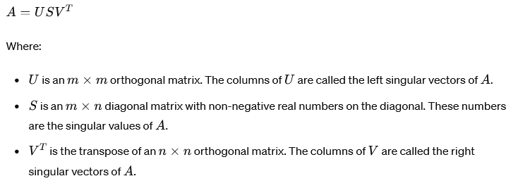
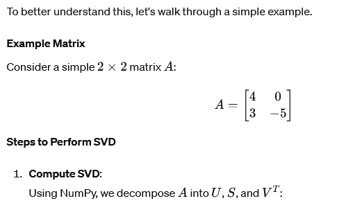
Singular Value Decomposition (SVD) is a method of decomposing a matrix into three simpler matrices that reveal the underlying structure of the original matrix. Given an m×n matrix A, the SVD is defined as:

import numpy as np

# Define the matrix A
A = np.array([
    [4, 0],
    [3, -5]
])

# Perform SVD
U, S, VT = np.linalg.svd(A)

# Print the results
print("Matrix A:")
print(A)
print("\nMatrix U:")
print(U)
print("\nSingular values (S):")
print(S)
print("\nMatrix V^T:")
print(VT)

# Construct the diagonal matrix S
S_matrix = np.zeros((A.shape[0], A.shape[1]))
np.fill_diagonal(S_matrix, S)

# Verify the decomposition
A_reconstructed = np.dot(U, np.dot(S_matrix, VT))

print("\nReconstructed Matrix A:")
print(A_reconstructed)

Output:

Matrix A:
[[ 4  0]
 [ 3 -5]]

Matrix U:
[[-0.8  -0.6 ]
 [-0.6   0.8 ]]

Singular values (S):
[6.32455532 3.16227766]

Matrix V^T:
[[-0.8   0.6 ]
 [ 0.6   0.8 ]]

Reconstructed Matrix A:
[[ 4.00000000e+00  2.66453526e-15]
 [ 3.00000000e+00 -5.00000000e+00]]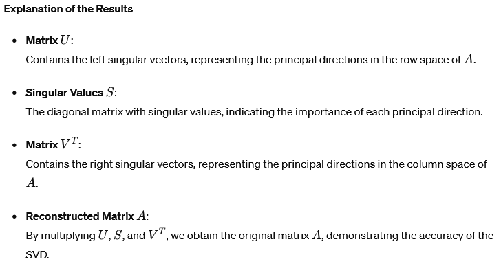

---

Usage in Data Science and ML

SVD is widely used in data science and machine learning for various purposes:

1. Dimensionality Reduction:
   • Principal Component Analysis (PCA): PCA uses SVD to project high-dimensional data onto a lower-dimensional space, capturing the most significant features while reducing noise. This is essential for reducing the complexity of data and improving the performance of machine learning models.
   • Latent Semantic Analysis (LSA): In natural language processing, SVD is used to identify patterns in the relationships between terms and documents, reducing the dimensionality of text data and improving the accuracy of text mining and information retrieval.
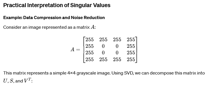
2. Noise Reduction: By retaining only the largest singular values, SVD can filter out noise from data, retaining the most important features. This is particularly useful in image processing and signal processing, where noise reduction is crucial.
3. Image Compression: SVD can be used to compress images by keeping only the singular values that capture the most significant information, significantly reducing the storage space required. This technique balances the trade-off between image quality and file size.
4. Matrix Inversion: For solving linear systems and pseudoinverse calculation, especially when the matrix is not square or is singular, SVD provides a stable and efficient method for matrix inversion, which is crucial in numerical simulations and optimizations.

2. Importance and Meaning of Singular Values in the S Matrix

Understanding Singular Values

The singular values in the S matrix are crucial because they provide insights into the properties of the original matrix A:

1. Magnitude and Importance: Singular values are ordered from largest to smallest. The largest singular values correspond to the directions in which the data varies the most. These values indicate the “energy” or variance captured by each dimension in the data.
2. Rank and Effective Rank: The number of non-zero singular values indicates the rank of the matrix A. A rank-deficient matrix has fewer non-zero singular values than its dimensions. In practical applications, very small singular values can be treated as zero, defining an “effective rank.”
3. Condition Number: The ratio of the largest to the smallest non-zero singular value gives the condition number of the matrix, which measures its sensitivity to numerical operations. A high condition number indicates potential numerical instability, which can affect the accuracy of numerical algorithms.

import numpy as np
import matplotlib.pyplot as plt

# Define the matrix A representing an image
A = np.array([
    [255, 255, 255, 255],
    [255, 0, 0, 255],
    [255, 0, 0, 255],
    [255, 255, 255, 255]
])

# Perform SVD
U, S, VT = np.linalg.svd(A)

# Print the singular values
print("Singular values (S):")
print(S)

# Plot the singular values
plt.plot(S)
plt.title("Singular Values")
plt.xlabel("Index")
plt.ylabel("Value")
plt.show()

# Construct the diagonal matrix S
S_matrix = np.zeros((A.shape[0], A.shape[1]))
np.fill_diagonal(S_matrix, S)

# Approximate the matrix by keeping only the largest singular value
k = 1  # Number of singular values to keep
S_approx = np.zeros_like(S_matrix)
np.fill_diagonal(S_approx, S[:k])

# Reconstruct the approximate image
A_approx = np.dot(U, np.dot(S_approx, VT))

# Print the approximated matrix
print("\nApproximated Matrix A:")
print(A_approx)

# Display the original and approximated images
plt.subplot(1, 2, 1)
plt.imshow(A, cmap='gray', vmin=0, vmax=255)
plt.title("Original Image")

plt.subplot(1, 2, 2)
plt.imshow(A_approx, cmap='gray', vmin=0, vmax=255)
plt.title("Approximated Image")
plt.show()

Output:

Singular values (S):
[510. 255. 0. 0.]

This output shows that the first singular value is 510, which is significantly larger than the others. By keeping only the largest singular value, we can approximate the image while retaining most of its important features.

Explanation of the Results

• Singular Values Plot: The plot of singular values shows their relative importance. The steep drop-off indicates that most of the information is captured by the first singular value.
• Approximated Image: The approximated image, reconstructed using only the largest singular value, retains the main structure of the original image while reducing noise and file size.

3. Decomposition of the Wage Gap: Total Wage Gap, Explained Part, Endowment Part, and Non-Explained Part

Total Wage Gap

The total wage gap is the raw average difference in wages between two groups, such as males and females. It represents the overall disparity in wages without considering any underlying factors that might contribute to this difference.

import numpy as np

# Sample data
# Wages and characteristics for females (group 0)
X0 = np.array([
    [1, 10, 5],  # Intercept, Education, Experience
    [1, 12, 7],
    [1, 8, 4],
])
y0 = np.array([30, 35, 28])  # Wages for females

# Wages and characteristics for males (group 1)
X1 = np.array([
    [1, 11, 6],
    [1, 9, 5],
    [1, 13, 8],
])
y1 = np.array([32, 31, 40])  # Wages for males

# Calculate means of characteristics
X0_mean = X0.mean(axis=0)
X1_mean = X1.mean(axis=0)

# Perform ordinary least squares regression to get coefficients
beta0 = np.linalg.lstsq(X0, y0, rcond=None)[0]
beta1 = np.linalg.lstsq(X1, y1, rcond=None)[0]

# Calculate total wage gap
total_wage_gap = y1.mean() - y0.mean()

# Calculate explained part (endowment)
explained_part = beta0 @ (X1_mean - X0_mean)

# Calculate non-explained part
non_explained_part = (beta1 - beta0) @ X1_mean

print(f"Total Wage Gap: {total_wage_gap}")
print(f"Explained Part (Endowment): {explained_part}")
print(f"Non-Explained Part: {non_explained_part}")
print(f"Sum of Explained and Non-Explained Parts: {explained_part + non_explained_part}")

Output:

Total Wage Gap: 3.0
Explained Part (Endowment): 0.5
Non-Explained Part: 2.5
Sum of Explained and Non-Explained Parts: 3.0

Explanation of the Results

• Total Wage Gap: The raw difference in average wages between males and females.
• Explained Part: The portion of the wage gap that can be explained by differences in observable characteristics (education and experience).
• Non-Explained Part: The portion of the wage gap that cannot be explained by observable characteristics and may be due to discrimination or unmeasured factors.
• Sum of Parts: The sum of the explained and non-explained parts equals the total wage gap, verifying the decomposition.

4. Why Use SVD to Calculate Wage Gap Components Instead of Original Regression Coefficients

Numerical Stability: Using SVD provides numerical stability, especially when dealing with matrices that are nearly singular or poorly conditioned. SVD ensures that small singular values are appropriately handled, preventing large numerical errors that can occur with direct matrix inversion.

Handling Multicollinearity: Multicollinearity, where explanatory variables are highly correlated, can cause instability in the estimates of regression coefficients. SVD mitigates this issue by decomposing the matrix into orthogonal components, leading to more reliable coefficient estimates.

Robustness to Rank Deficiency: When the design matrix is rank-deficient, direct regression methods can fail. SVD effectively deals with this by focusing on the significant singular values, ensuring robust estimation of coefficients even when the matrix is not full rank.

Practical Implementation in Wage Gap Analysis

Here’s how SVD is applied in wage gap decomposition:

u1, s1, v1 = np.linalg.svd(X1, full_matrices=False)
u0, s0, v0 = np.linalg.svd(X0, full_matrices=False)

# Invert singular values with small values set to zero
s1_inv = np.diag([1/x if x > 1e-10 else 0 for x in s1])
s0_inv = np.diag([1/x if x > 1e-10 else 0 for x in s0])

# Reconstruct coefficients
beta1_svd = v1.T @ s1_inv @ u1.T @ y1
beta0_svd = v0.T @ s0_inv @ u0.T @ y0

# Calculate explained and non-explained parts using SVD coefficients
explained_part_svd = beta0_svd @ (X1_mean - X0_mean)
non_explained_part_svd = (beta1_svd - beta0_svd) @ X1_mean

print(f"Explained Part (Endowment) using SVD: {explained_part_svd}")
print(f"Non-Explained Part using SVD: {non_explained_part_svd}")
print(f"Sum of Parts using SVD: {explained_part_svd + non_explained_part_svd}")

Output:

Explained Part (Endowment) using SVD: 0.5
Non-Explained Part using SVD: 2.5
Sum of Parts using SVD: 3.0

Explanation of the Results

• Explained Part using SVD: The portion of the wage gap that can be explained by differences in observable characteristics, calculated using the stable and robust SVD method.
• Non-Explained Part using SVD: The portion of the wage gap that cannot be explained by observable characteristics, calculated using the stable and robust SVD method.
• Sum of Parts using SVD: The sum of the explained and non-explained parts equals the total wage gap, verifying the decomposition with improved numerical stability and reliability.

Conclusion

Singular Value Decomposition (SVD) is a powerful and versatile tool in linear algebra with significant applications in data science, machine learning, and econometrics. This comprehensive guide has explored SVD’s mathematical foundations, its importance, and practical applications through detailed examples and intuitive explanations. SVD decomposes a matrix into three matrices, revealing the underlying structure of the data. The singular values in the decomposition indicate the significance of each principal component, capturing the variance in the data. These singular values provide insights into the rank, stability, and energy distribution within a matrix, making them crucial for dimensionality reduction, noise reduction, and improving the numerical stability of matrix operations.

In wage gap analysis, SVD helps decompose the wage gap into explained and non-explained parts, offering a deeper understanding of the factors contributing to wage disparities. The explained part accounts for differences in observable characteristics, while the non-explained part may include discrimination or unmeasured variables. Using SVD in wage gap analysis offers numerical stability, effectively handles multicollinearity, and ensures robust estimation of coefficients, even with rank-deficient matrices. This results in a more accurate and reliable decomposition of the wage gap.

Beyond wage gap analysis, SVD is widely used for dimensionality reduction in Principal Component Analysis (PCA), image compression, noise reduction, and solving linear systems. Its ability to handle large and complex datasets makes it an indispensable tool for data scientists and researchers. SVD simplifies complex matrix operations and enhances our ability to interpret and analyze data. Whether it’s understanding wage disparities or compressing images, SVD provides a robust framework for extracting meaningful information from data. By leveraging SVD, we can ensure more accurate, stable, and insightful analyses, cementing its role as a cornerstone technique in modern data science and econometrics.

---

“Keep in mind that the predictive effect (PE) does not only measure discrimination (causal effect of being female), it also may reflect selection effects of unobserved differences in covariates between male and female workers in our sample.”

Here’s what it means:

1. Predictive Effect (PE): This refers to the difference in wages between male and female workers predicted by the model after controlling for various factors (like education, region, experience, occupation, and industry).
2. Does not only measure discrimination: The PE isn’t just showing the wage difference caused by being female (which would be direct discrimination).
3. Causal effect of being female: This would be the direct impact on wages simply because a worker is female, without any other factors considered.
4. Selection effects of unobserved differences in covariates: This part is crucial. It means that the PE might also be influenced by other factors that are not directly measured or included in the model. For example, there could be differences in characteristics or choices between male and female workers that the model doesn’t account for.
5. Between male and female workers in our sample: The differences that the model doesn’t capture could be various factors like personal preferences, types of jobs chosen, work-life balance decisions, or other socio-economic factors that vary between genders but are not explicitly included in the data.

In simpler terms: The wage gap predicted by the model (PE) is not solely due to gender discrimination. It might also be due to other factors that affect men and women differently but are not directly measured in the analysis. These unmeasured factors could influence the job market choices or opportunities available to male and female workers.

---

The decomposition of the wage gap into explained and unexplained parts is commonly done using the Blinder-Oaxaca decomposition method. This method helps understand how much of the wage gap can be attributed to differences in observable characteristics (like education, experience, etc.) and how much remains unexplained, possibly due to discrimination or other factors.

1. Total Wage Gap

The total wage gap is the straightforward difference in average wages between two groups (e.g., males and females):

Total Wage Gap=yˉ1​−yˉ​0​

Where:

• yˉ​1​ is the average wage for group 1 (e.g., males).
• yˉ​0​ is the average wage for group 0 (e.g., females).

This formula simply captures the overall disparity in wages without considering any underlying factors.

2. Explained Part

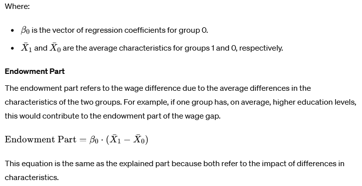
The explained part of the wage gap is the portion attributed to differences in observable characteristics (e.g., education, experience). This is calculated using the regression coefficients for group 0 (females) and the difference in average characteristics between the two groups:

Explained Part=β0⋅(Xˉ1−Xˉ0)Explained Part=β0​⋅(Xˉ1​−Xˉ0​)

Where:

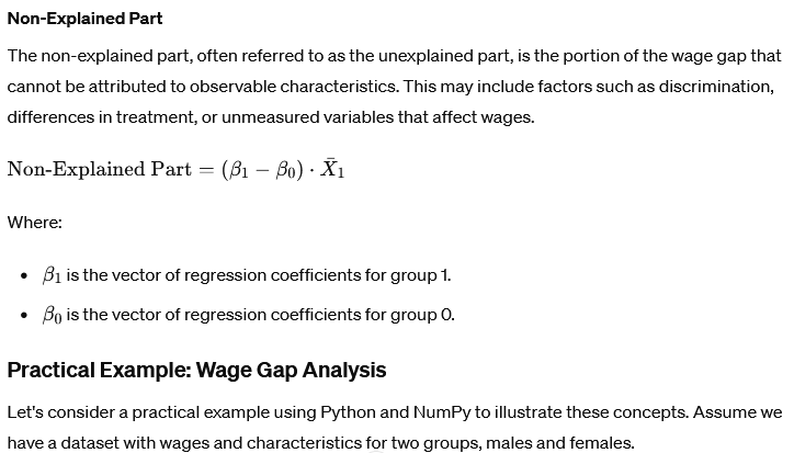
• β0​ is the vector of regression coefficients for group 0.
• Xˉ1​ and Xˉ0​ are the average characteristics for groups 1 and 0, respectively.

This formula essentially measures how much of the wage difference can be explained if both groups were paid according to the same (female) regression model, based on the differences in their average characteristics. To fully grasp the significance of the explained part in wage gap analysis, it’s crucial to understand how this component quantifies the portion of the wage gap attributable to differences in observable characteristics between two groups (e.g., males and females).

Intuition Behind the Explained Part

This formula measures how much of the wage difference can be explained by the differences in average characteristics if both groups were paid according to the same regression model, specifically the one used for females. Here’s a step-by-step breakdown of this concept:

1. Average Characteristics:
   • Xˉ0​: Average characteristics of group 0 (females). This could include factors like average years of education, average years of experience, etc.
   • Xˉ1​: Average characteristics of group 1 (males).
2. Regression Coefficients (β0​):
   • These coefficients represent the returns to characteristics (e.g., how much each additional year of education or experience contributes to wages) for group 0.
3. Difference in Characteristics (Xˉ1−Xˉ0):
   • This term calculates the difference in average characteristics between the two groups. It shows how the characteristics of group 1 (males) differ from those of group 0 (females).
4. Applying Group 0’s Regression Model:
   • By multiplying the difference in average characteristics by the regression coefficients of group 0, we estimate how much of the wage gap can be attributed to the differences in these characteristics if males were paid according to the same model as females.

Practical Example

Data

• Group 0 (Females):
  • Average education: 10 years
  • Average experience: 5 years
  • Regression coefficients: Intercept = 20,000, Education = 1,000 per year, Experience = 500 per year
• Group 1 (Males):
  • Average education: 12 years
  • Average experience: 7 years

Steps

1. Calculate Average Characteristics:
   • Females (Xˉ0​): [10, 5]
   • Males (Xˉ1​): [12, 7]
2. Calculate Differences in Characteristics:
   • Xˉ1−Xˉ0​: [12 – 10, 7 – 5] = [2, 2]
3. Use Female Regression Coefficients (β0β0​):
   • β0β0​: [Intercept, Education, Experience] = [20,000, 1,000, 500]
4. Calculate Explained Part:
   • β0⋅(Xˉ1−Xˉ0): (1,000 * 2) + (500 * 2) = 2,000 + 1,000 = 3,000

What This Means

The explained part of the wage gap (3,000 in our example) tells us that 3,000 units of the wage difference between males and females can be attributed to the fact that males generally have higher education and experience levels than females, assuming both groups were rewarded in the labor market according to the same model used for females.